In this tutorial, we will build an image classification Deep Learning model using the torch R package. The dataset for this tutorial is the Dataset of Vector Mosquito Images published by Pise and contributors in Mendeley Data (DOI:10.17632/88s6fvgg2p.4). We downloaded the Mosquito Images Augmented.zip for the purposes of this tutorial.

By the end of this tutorial, you should be able to:

load and preprocess your own images into torch tensors
import a prebuilt Artificial Neural Network architecture
fit an Artificial Neural Network model to your data
evaluate a deep learning model
draw inference on a new image (predict a mosquito specie from an image) and
deploy the image classification model as a shiny app

This tutorial is inspired by the Classifying images with torch tutorial by Sigrid Keydana.

We first load the tidyverse package, then load the torch, torchvision, and luz packages which are all part of the mlverse, a collection of open source libraries to scale Data Science.

All packages are published on the Comprehensive R Archive Network (CRAN) and can therefore be installed with the install.packages() function provided by base R.

library(tidyverse)
library(torch)
library(torchvision)
library(luz)

We use the shiny R package for model deployment (run install.packages("shiny") from your R console to install shiny).

Let’s set a seed for R and torch for reproducible results:

set.seed(1234)
torch_manual_seed(1234)

Unzipping the images

After moving the Mosquito Images Augmented.zip archive to our working directory, we unzip the image files into a folder named mosquitospecies as follows:

unzip("Mosquito Images Augmented.zip", exdir = "mosquitospecies")

root_dir <- file.path(getwd(), "mosquitospecies")

Let’s identify and clean out corrupt image files.

deleted_files <- 0
for(path in list.files(root_dir, recursive = TRUE, full.names = TRUE)){
  img <- try(jpeg::readJPEG(path), silent = TRUE)
  if(any(class(img) == "try-error")){
    print(path)
    file.remove(path)
    deleted_files <- deleted_files + 1
  }
}
cli::cli_alert(
  paste(deleted_files, "corrupt files have been identified and deleted.")
)

Data Loading and preprocessing

We check for GPU acceleration and use it whenever available.

# Check for GPU accelaration
device <- if (cuda_is_available()) torch_device("cuda:0") else "cpu"

Image Preprocessing

On the training set, most of the preprocessing involves image standardization, augmenting the data by adding noise, and normalization to comply with the ResNet Artificial Neural Network architecture (often used for image classification) which we use in this tutorial.

# Define Image transformation helper function
train_transform <- function(img) {
  img %>%
    transform_to_tensor() %>%
    (function(x) x$to(device = device)) %>%
    transform_color_jitter() %>%
    transform_random_horizontal_flip() %>%
    transform_normalize(
      mean = c(0.485, 0.456, 0.406), 
      std = c(0.229, 0.224, 0.225)
    )
}

For the validation and test sets, no noise was introduced in the data. Images are resized, and normalized accordingly.


test_transform <- valid_transform <- function(img) {
  img %>%
    transform_to_tensor() %>%
    (function(x) x$to(device = device)) %>%
    transform_normalize(
      mean = c(0.485, 0.456, 0.406), 
      std = c(0.229, 0.224, 0.225)
    )
}

To import and generate the image dataset for torch, we create the mosquitospecies_dataset utility which inherits from the torchvision::image_folder_dataset dataset utility generator.

# Define Cats and Dogs dataset model
mosquitospecies_dataset <- dataset(
  "mosquitospecies_folder",
  inherit = torchvision::image_folder_dataset,
  initialize = function(root, indices, transform=NULL, target_transform=NULL,
                        loader=NULL, is_valid_file=NULL) {
    super$initialize(root, transform=transform,
                     target_transform=target_transform, loader = loader,
                     is_valid_file=is_valid_file)
    self$indices <- indices
  },
  .getitem = function(index) {
    
    path <- self$samples[[1]][self$indices[index]]
    target <- self$samples[[2]][self$indices[index]]
    
    sample <- self$loader(path)
    
    if (!is.null(self$transform))
      sample <- self$transform(sample)
    
    if (!is.null(self$target_transform))
      target <- self$target_transform(target)
    
    list(x = sample, y = target)
  },
  .length = function() {
    length(self$indices)
  }
)

Now, let’s randomly split the data into training (70%), validation (20%), and test (10%) sets:

num_imgs <- length(list.files(root_dir, recursive = TRUE))
train_indices <- sample(1:num_imgs, num_imgs * 0.7)
valid_indices <- sample(setdiff(1:num_imgs, train_indices), num_imgs*0.2)
test_indices <- setdiff(setdiff(1:num_imgs, train_indices), valid_indices)

Now, we use the dataset generator utility to create the training set and the validation set.

train_ds <- mosquitospecies_dataset(root_dir, train_indices, transform = train_transform)
train_ds$.length()
#> [1] 1847

valid_ds <- mosquitospecies_dataset(root_dir, valid_indices, transform = valid_transform)
valid_ds$.length()
#> [1] 528

test_ds <- mosquitospecies_dataset(root_dir, test_indices, transform = test_transform)
test_ds$.length()
#> [1] 265

The generated datasets contain 1847, 528 and 265 images data respectively for the training, validation and test sets.

Let’s check whether each set contains the same number of classes:

length(train_ds$classes)
length(valid_ds$classes)
length(test_ds$classes)
class_names <- test_ds$classes

cli::cli_alert(paste0(length(class_names), " classes identified. Classes are: ", paste(class_names, collapse = ", "),"."))

Good news, our classes are equally represented in the training, validation and training sets.

Data Loader

We create a dataloader for each set with a batch size of 16 images.

batch_size <- 16

train_dl <- dataloader(train_ds, batch_size = batch_size, shuffle = TRUE)
valid_dl <- dataloader(valid_ds, batch_size = batch_size)
test_dl <- dataloader(test_ds, batch_size = batch_size)

Let’s check the number of batches in each loader:

train_dl$.length() 
#> [1] 116

valid_dl$.length() 
#> [1] 33

test_dl$.length()  
#> [1] 17

Visualizing the data

Here, we visualize the 16 images in the first batch of the training set.

b <- train_dl$.iter()$.next() # take one batch in the training set
targets <- b$y

images <- b$x %>% 
  as_array() %>% 
  aperm(perm = c(1, 3, 4, 2))

mean <- c(0.485, 0.456, 0.406)
std <- c(0.229, 0.224, 0.225)
images <- std * images + mean
images <- images * 255
images[images > 255] <- 255
images[images < 0] <- 0

par(mfcol = c(4,4), mar = rep(1, 4))

images %>%
  array_tree(1) %>%
  set_names(class_names[as_array(targets)]) %>%
  map(as.raster, max = 255) %>%
  iwalk(~{plot(.x); title(.y)})

Classifying Mosquitoes by Species - the Model

We use the ResNet Artificial Neural Network architecture which is often used for image classification. We replace the output layer of the architecture to match our number of classes, which is 3 in this tutorial.

We also use the cross entropy loss as our loss function, and choose the Adam optimizer to update the parameters (weights and biases) of the model in order to minimize the loss function during the training process.

model <- model_resnet18(pretrained = TRUE)

model$parameters %>% purrr::walk(function(param) param$requires_grad_(FALSE))

model$fc <- nn_linear(in_features = model$fc$in_features, out_features = length(class_names))

model <- model$to(device = device)

criterion <- nn_cross_entropy_loss()

optimizer <- optim_adam(model$parameters, lr = 0.05)

To make sure that we have all shapes matching up, let’s call the model on a batch of our data:

model(b$x)

#> torch_tensor
#>  0.2884 -0.9359  1.3895
#> -0.0359 -0.2018  0.8943
#>  0.5630 -1.4051  0.7087
#>  0.3417 -0.6062  0.8235
#>  0.4191 -1.5016  1.2196
#>  0.4454 -1.7770 -0.0628
#>  0.7498 -1.6461  0.7906
#>  1.2950 -1.5470  0.9477
#> -0.0840 -1.0470  0.8228
#>  1.0521 -0.8955  0.1835
#>  0.2959 -1.0010  1.1621
#>  0.4893 -0.8946  0.7766
#>  0.2516 -1.3598  1.1719
#>  0.0574 -0.4127  0.9373
#> -0.2904 -0.8852  1.3795
#>  0.8048 -1.8014 -0.1916
#> [ CPUFloatType{16,3} ][ grad_fn = <AddmmBackward0> ]

Let’s instantiate the scheduler:

num_epochs = 10

scheduler <- optimizer %>% 
  lr_one_cycle(max_lr = 0.05, epochs = num_epochs, steps_per_epoch = train_dl$.length())

Train the Model

train_batch <- function(b) {
  
  optimizer$zero_grad()
  output <- model(b$x)
  loss <- criterion(output, b$y$to(device = device))
  loss$backward()
  optimizer$step()
  scheduler$step()
  loss$item()
  
}

valid_batch <- function(b) {
  
  output <- model(b$x)
  loss <- criterion(output, b$y$to(device = device))
  loss$item()
}

for (epoch in 1:num_epochs) {
  
  model$train()
  train_losses <- c()
  
  coro::loop(for (b in train_dl) {
    loss <- train_batch(b)
    train_losses <- c(train_losses, loss)
  })
  
  model$eval()
  valid_losses <- c()
  
  coro::loop(for (b in valid_dl) {
    loss <- valid_batch(b)
    valid_losses <- c(valid_losses, loss)
  })
  
  cat(
    sprintf("\nLoss at epoch %d: training: %3f, validation: %3f\n", 
      epoch, mean(train_losses), mean(valid_losses))
  )
}
#> 
#> Loss at epoch 1: training: 0.691431, validation: 0.347098
#> 
#> Loss at epoch 2: training: 0.801611, validation: 2.819351
#> 
#> Loss at epoch 3: training: 1.176880, validation: 0.266920
#> 
#> Loss at epoch 4: training: 1.017648, validation: 3.553514
#> 
#> Loss at epoch 5: training: 1.211209, validation: 0.210213
#> 
#> Loss at epoch 6: training: 0.957843, validation: 0.179759
#> 
#> Loss at epoch 7: training: 0.495530, validation: 0.457704
#> 
#> Loss at epoch 8: training: 0.305884, validation: 0.217924
#> 
#> Loss at epoch 9: training: 0.419141, validation: 0.354136
#> 
#> Loss at epoch 10: training: 0.242781, validation: 0.189291

Test set accuracy

We assess the accuracy of the model by evaluating it on the test set as follows:

model$eval()

test_losses <- c()
total <- 0
correct <- 0

test_batch <- function(b) {
  
  output <- model(b$x)
  labels <- b$y$to(device = device)
  loss <- criterion(output, labels)
  
  test_losses <<- c(test_losses, loss$item())
  predicted <- torch_max(output$data(), dim = 2)[[2]]
  total <<- total + labels$size(1)
  correct <<- correct + (predicted == labels)$sum()$item()
  
}

coro::loop(for (b in test_dl) {
  test_batch(b)
})

mean(test_losses)
#> [1] 0.2414807

We therefore calculate the accuracy of our model:

test_accuracy <-  correct/total
test_accuracy
#> [1] 0.9509434

Impressive, our model correctly identifies the correct species 95.1% of the time.

Run inference on new image

Let’s put our newly built model to the task by predicting the species of a mosquito from its image. For this task, we choose a new image and try to predict the mosquito species in the image.

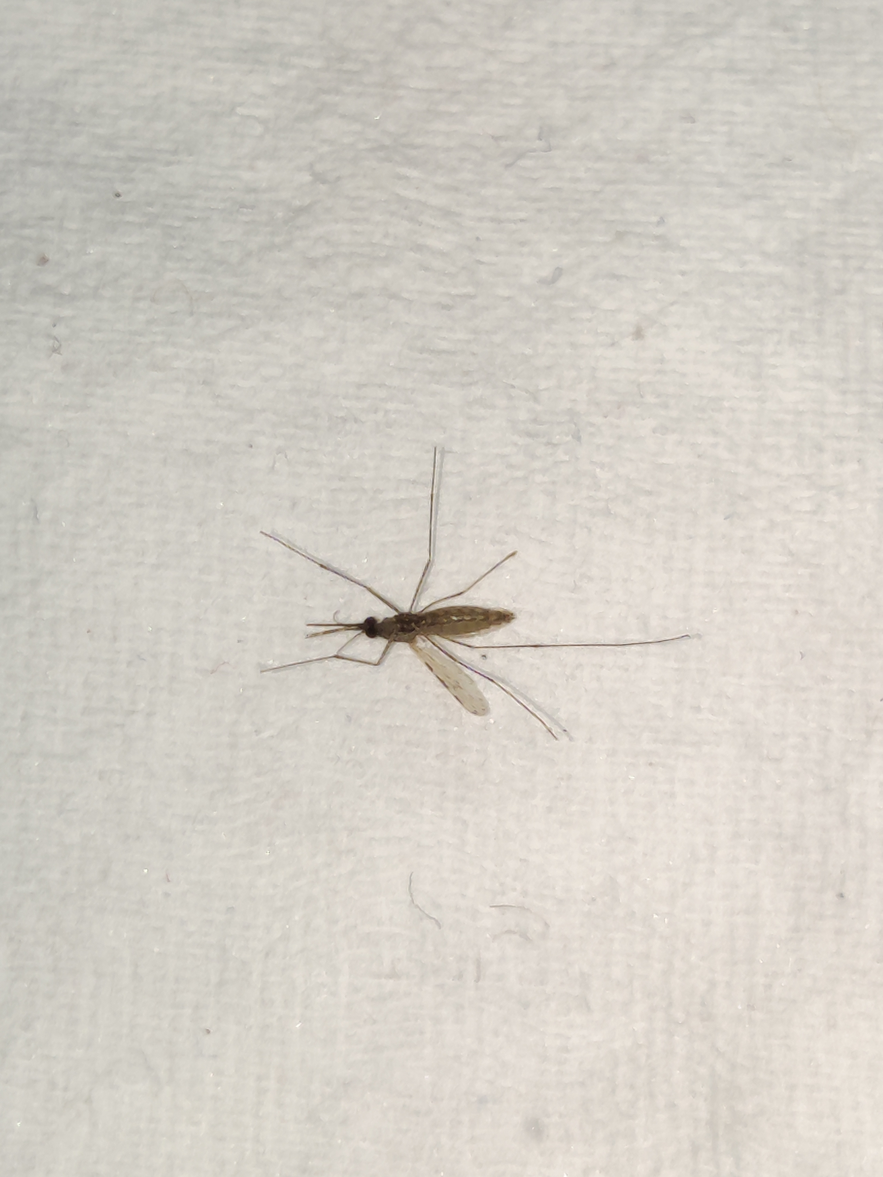
The above picture has a 3000 by 4000 picture which was not included in the training, testing or even the validation set. We know that the mosquito in the picture belongs to the Anopheles stephensi species.

To predict new images, we write the function below which takes an image path, a model, and a class names vector, and output the predicted class name:

predict_species <- function(path, dl_model = model, all_classes = class_names){
  img_tensor <- path %>% 
    jpeg::readJPEG() %>% 
    transform_to_tensor() %>%
    (function(x) x$to(device = device)) %>% 
    transform_resize(size = c(256, 256)) %>% 
    transform_normalize(
      mean = c(0.485, 0.456, 0.406), 
      std = c(0.229, 0.224, 0.225)
    )
  
  prediction <- img_tensor$unsqueeze(dim = 1) %>% 
    dl_model() %>% 
    torch_max(dim = 2)
  
  all_classes[prediction[[2]] %>% as.numeric]
}

We now use the custom function defined above to predict the species of the mosquito in the picture above:

predict_species("unknown_mosquito_species.jpg")
#> [1] "Anopheles Stephensi"

Our model accurately predicts that the species of the mosquito in the picture above is Anopheles stephensi.

Let’s save our model for a future deployment:

torch_save(model, "mosquito_class_model.rt")

Deployment

We deploy the image classification model built in this tutorial as a small shiny app. You may run it from an R console with the following R script:

shiny::runGitHub("mosquitoImageClassification", "rosericazondekon")

Conclusion

In this tutorial, we built a Deep Learning model to draw inference on a specie of a mosquito given its image. The model’s performance can be improved by training with a lower learning rate, or increasing the training epochs. Our model is quite limitted as it can only identifies 3 different species of mosquitoes. A large dataset from a large number of mosquito species would be an interesting project to pursue. The deployment of a more capable model (as a webapp or a smartphone app) may supplement morphological keys in the identification of mosquito species. Furthermore, such a tool may serve as an important leverage to entomologic surveillance programs and systems particularly in countries where mosquito vector-borne diseases are endemic.

Mosquito Species Image Classification using the torch R package